
Forecast Volatility for 0DTE options the right way!
Using the RVRP-Adjusted VIX1D

Welcome to my first post, which will be about adjusting the VIX1D to get a better volatility forecast, which can be used with short-term options trading.
Introduction to VIX1D
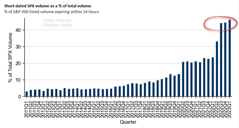
The VIX1D was launched not so long ago on April 2023. According to Goldman Sachs, the proportion of 0DTE options in the total trading volume of all SPX options has doubled since 2022, now exceeding 40% of the market. With the VIX1D, 0DTE trading is easier (or is it….?) as we can make more informed decisions regarding expected volatility within the trading day rather than using the VIX, which measures 30-day expected volatility. The VIX is by far one of the most popular market indices and has been proven to enhance volatility forecasts, but not really for 0DTE, because it uses prices of options with a remaining maturity between 23 and 37 days to the Friday SPX expiration. Whereas, VIX1D includes 0DTE options in its calculations.
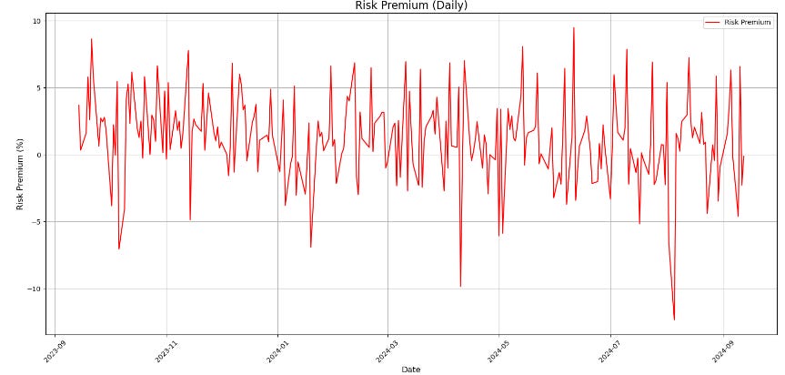
The Volatility Risk Premium (VRP) Issue
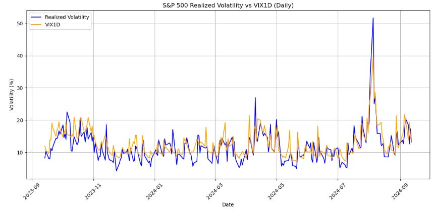
Options are primarily used for hedging. As options are bought to hedge downside protection on the indices, this leads to an increase in implied volatility which is the reason why implied volatility is priced above realized volatility a lot of the time, which is evident in the image above. This overestimation of volatility is what creates the Volatility Risk Premium (VRP). There are many ways to harvest this Volatility Risk Premium, such as selling options and profiting from theta decay, which will be mentioned in a post later. To address this issue, you can implement the Realized Volatility Risk Premium (RVRP) adjusted VIX1D forecast mentioned in the paper by Albers (2023)1.
RVRP-Adjusted VIX1D Forecasts
There are three RVRP-Adjusted VIX1D Forecast methods:
Adjusting using the most recent RVRP:
\(\widehat{R V}_t^{R V R P}=V I X 1 D_{t-1}-R V R P_{t-1}\)Adjusting using the mean RVRP over the last 21 trading days:
\(\widehat{R V}_t^{\text {mean } R V R P}=V I X 1 D_{t-1}-\frac{1}{21} \sum_{i=1}^{21} R V R P_{t-i},\)Adjusting using the median RVRP over the last 21 trading days:
\(\widehat{R V}_t^{\text {med } R V R P}=V I X 1 D_{t-1}-\text { median }\left(R V R P_{t-1}, \ldots, R V R P_{t-21}\right)\)
Firstly to calculate realized volatility we will use the equation:
where rt,i is the ith logarithmic return on day t and Mt denotes the number of five-minutes returns of day t. RVt refers to the realized volatility.
Now lets implement this in Python
Packages
import requests
import pandas as pd
import numpy as np
import matplotlib.pyplot as plt
from datetime import datetime, timedelta
import pandas_market_calendars as mcal
from sklearn.metrics import mean_squared_error, mean_absolute_error
Fetching data
We will be using Polygon API for our data for the VIX1D and SPY. There is a limit of amount of data you can fetch in one request so we will fetch the data in batches.
API_KEY = "INSERT YOUR API KEY"

# Set the parameters for the API request
sp500_ticker = "SPY"
vix1d_ticker = "I:VIX1D"
end_date = datetime.now()
start_date = end_date - timedelta(days=365)

# Format dates for the API request
start_str = start_date.strftime("%Y-%m-%d")
end_str = end_date.strftime("%Y-%m-%d")

def get_data(ticker, start_date, end_date, multiplier=5, timespan='minute'):
    url = f"https://api.polygon.io/v2/aggs/ticker/{ticker}/range/{multiplier}/{timespan}/{start_date}/{end_date}?adjusted=true&sort=asc&limit=50000&apiKey={API_KEY}"
    response = requests.get(url)

    if response.status_code == 200:
        data = response.json().get('results', [])
        return pd.DataFrame(data)
    else:
        print(f"Error fetching data for {ticker}: {response.status_code}")
        return None

def fetch_data_in_chunks(ticker, start_date, end_date, chunk_size=7):
    all_data = pd.DataFrame()
    current_start = start_date

    while current_start < end_date:
        current_end = min(current_start + timedelta(days=chunk_size), end_date)
        print(f"Fetching data from {current_start} to {current_end}")
        chunk_data = get_data(ticker, current_start.strftime("%Y-%m-%d"), current_end.strftime("%Y-%m-%d"))

        if chunk_data is not None and not chunk_data.empty:
            all_data = pd.concat([all_data, chunk_data])

        current_start = current_end + timedelta(days=1)

    return all_data

# Fetch data in chunks for SPY and VIX1D
sp500_data = fetch_data_in_chunks(sp500_ticker, start_date, end_date)
vix1d_data = fetch_data_in_chunks(vix1d_ticker, start_date, end_date)
Plotting the realized volatility and VIX1D daily and calculating MSE, MAE and MAPE
if sp500_data is not None and vix1d_data is not None:
    # Calculate the log difference of closing prices (log returns)
    sp500_data['timestamp'] = pd.to_datetime(sp500_data['t'], unit='ms')
    sp500_data['c_log_diff'] = np.log(sp500_data['c']) - np.log(sp500_data['c'].shift(1))

    # Define a function to calculate realized volatility using the c_log_diff method
    def calculate_realized_volatility(df):
        """
        Calculate realized volatility for each day using log differences.
        """
        realized_vol = (df['c_log_diff'] ** 2).sum()  # Sum of squared log differences
        realized_vol = np.sqrt(realized_vol) * 100 * np.sqrt(252)  # Annualizing the volatility
        return realized_vol

    # Add a column for 'date' to group by
    sp500_data['date'] = sp500_data['timestamp'].dt.date

    # Group by each trading day and calculate daily realized volatility
    daily_realized_volatility = sp500_data.groupby('date').apply(calculate_realized_volatility)
    daily_realized_volatility = pd.DataFrame(daily_realized_volatility, columns=['realized_volatility'])

    # Process VIX1D data
    vix1d_data['timestamp'] = pd.to_datetime(vix1d_data['t'], unit='ms')
    vix1d_data['date'] = vix1d_data['timestamp'].dt.date

    # Group VIX1D by date and take the daily close
    vix1d_daily = vix1d_data.groupby('date')['c'].last()
    vix1d_daily = pd.DataFrame(vix1d_daily)

    # Ensure both DataFrames have datetime.date as index
    daily_realized_volatility.index = pd.to_datetime(daily_realized_volatility.index).date
    vix1d_daily.index = pd.to_datetime(vix1d_daily.index).date

    # Merge realized volatility and VIX1D data
    merged_data = pd.merge(daily_realized_volatility, vix1d_daily, left_index=True, right_index=True)
    merged_data.columns = ['realized_volatility', 'vix1d']

    if not merged_data.empty:
        # Calculate MAPE
        mape = np.mean(np.abs((merged_data['realized_volatility'] - merged_data['vix1d']) / merged_data['realized_volatility'])) * 100
        mse = np.mean((merged_data['realized_volatility'] - merged_data['vix1d'])**2)

    # Calculate MAE
        mae = np.mean(np.abs(merged_data['realized_volatility'] - merged_data['vix1d']))
        # Get the NYSE calendar and filter out non-trading days
        nyse = mcal.get_calendar('NYSE')
        schedule = nyse.schedule(start_date=start_date, end_date=end_date)
        trading_days = schedule.index.date

        # Filter merged data to only include trading days
        merged_data = merged_data.loc[merged_data.index.isin(trading_days)]

        # Plot the data
        plt.figure(figsize=(12, 6))
        plt.plot(merged_data.index, merged_data['realized_volatility'], label='Realized Volatility', color='blue')
        plt.plot(merged_data.index, merged_data['vix1d'], label='VIX1D', color='orange')
        plt.title("S&P 500 Realized Volatility vs VIX1D (Daily)")
        plt.xlabel("Date")
        plt.ylabel("Volatility (%)")
        plt.legend()
        plt.grid(True)
        plt.xticks(rotation=45)
        plt.tight_layout()
        plt.show()
        plt.savefig('plot1.png')


        print(f"Mean Squared Error (MSE): {mse:.4f}")
        print(f"Mean Absolute Error (MAE): {mae:.4f}")
        print(f"Mean Absolute Percentage Error (MAPE): {mape:.2f}%")
    else:
        print("Merged data is empty. Check the indices and date ranges.")
else:
    print("Failed to retrieve data. Please check your API key and try again.")
Results for VIX1D

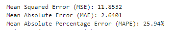
These are our evaluation metrics. We can come back to this as we compare it to the RVRP-Adjusted VIX1D forecast!
Plotting the RVRP-Adjusted VIX1D forecasts
# Calculate RVRP
merged_data['RVRP'] = merged_data['vix1d'].shift(1) - merged_data['realized_volatility']

# Calculate RVRP-adjusted VIX1D forecasts
merged_data['VIX1D_RVRP'] = merged_data['vix1d'].shift(1) - merged_data['RVRP'].shift(1)
merged_data['VIX1D_mean_RVRP'] = merged_data['vix1d'].shift(1) - merged_data['RVRP'].rolling(window=21).mean().shift(1)
merged_data['VIX1D_median_RVRP'] = merged_data['vix1d'].shift(1) - merged_data['RVRP'].rolling(window=21).median().shift(1)

# Remove rows with NaN values
merged_data_clean = merged_data.dropna()

# Create the plot
plt.figure(figsize=(16, 8))
plt.plot(merged_data_clean.index, merged_data_clean['realized_volatility'], label='Realized Volatility', color='blue')
plt.plot(merged_data_clean.index, merged_data_clean['VIX1D_RVRP'], label='VIX1D-RVRP', color='red')
plt.plot(merged_data_clean.index, merged_data_clean['VIX1D_mean_RVRP'], label='VIX1D-mean RVRP', color='green')
plt.plot(merged_data_clean.index, merged_data_clean['VIX1D_median_RVRP'], label='VIX1D-median RVRP', color='orange')

plt.title("Realized Volatility vs RVRP-adjusted VIX1D Forecasts", fontsize=16)
plt.xlabel("Date", fontsize=12)
plt.ylabel("Volatility (%)", fontsize=12)
plt.legend(fontsize=10)
plt.grid(True)
plt.xticks(rotation=45)
plt.tight_layout()
plt.show()

# Calculate MSE, MAE, and MAPE for each forecast
for forecast in ['VIX1D_RVRP', 'VIX1D_mean_RVRP', 'VIX1D_median_RVRP']:
    mse = mean_squared_error(merged_data_clean['realized_volatility'], merged_data_clean[forecast])
    mae = mean_absolute_error(merged_data_clean['realized_volatility'], merged_data_clean[forecast])
    mape = np.mean(np.abs((merged_data_clean['realized_volatility'] - merged_data_clean[forecast]) / merged_data_clean['realized_volatility'])) * 100

    print(f"\nMetrics for {forecast}:")
    print(f"MSE: {mse:.4f}")
    print(f"MAE: {mae:.4f}")
    print(f"MAPE: {mape:.2f}%")
Results for the RVRP-Adjusted VIX1D forecasts
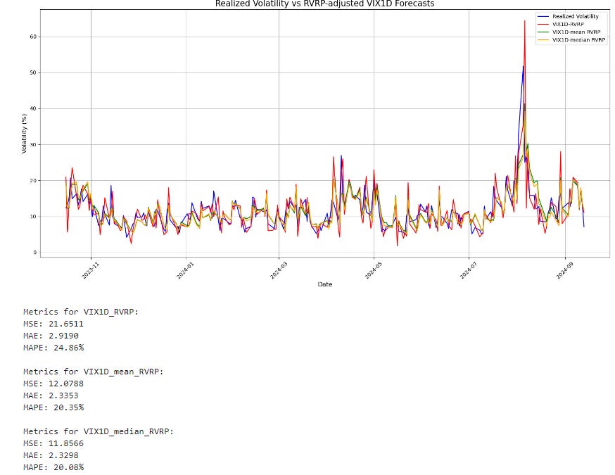
As we can see, the RVRP-Adjusted VIX1D forecast has better metrics than the standard VIX1D index. We can see that specifically taking the median of the last 21 days for the RVRP and adjusting the VIX1D we get the best results with the lowest MSE, MAE and MAPE values.
Albers, S. (2023a) ‘A new star is born: Does the VIX1D render common volatility forecasting models for the U.S. Equity Market Obsolete?’, SSRN Electronic Journal [Preprint]. doi:10.2139/ssrn.4505785.
Very informative, looking forward to further posts.